Panels

• 1: Line plots
• 1.1: Line plot reference
• 1.2: Point aggregation
• 1.3: Smooth line plots
• 2: Bar plots
• 3: Parallel coordinates
• 4: Scatter plots
• 5: Save and diff code
• 6: Parameter importance
• 7: Compare run metrics
• 8: Query panels
• 8.1: Embed objects

Use workspace panel visualizations to explore your logged data by key, visualize the relationships between hyperparameters and output metrics, and more.

Workspace modes

W&B projects support two different workspace modes. The icon next to the workspace name shows its mode.

Icon	Workspace mode
	Automated workspaces automatically generate panels for all keys logged in the project. Choose an automatic workspace: To get started quickly by visualizing all available data for the project. For a smaller projects that log fewer keys. For more broad analysis. If you delete a panel from an automatic workspace, you can use Quick add to recreate it.
	Manual workspaces start as blank slates and display only those panels intentionally added by users. Choose a manual workspace: When you care mainly about a fraction of the keys logged in the project. For more focused analysis. To improve the performance of a workspace, avoiding loading panels that are less useful to you. Use Quick add to easily populate a manual workspace and its sections with useful visualizations rapidly.

To change how a workspace generates panels, reset the workspace.

Undo changes to your workspace

To undo changes to your workspace, click the Undo button (arrow that points left) or type CMD + Z (macOS) or CTRL + Z (Windows / Linux).

Reset a workspace

To reset a workspace:

1. At the top of the workspace, click the action menu ....
2. Click Reset workspace.

Configure the workspace layout

To configure the workspace layout, click Settings near the top of the workspace, then click Workspace layout.

• Hide empty sections during search (turned on by default)
• Sort panels alphabetically (turned off by default)
• Section organization (grouped by first prefix by default). To modify this setting:
  1. Click the padlock icon.
  2. Choose how to group panels within a section.

To configure defaults for the workspace’s line plots, refer to Line plots.

Configure a section’s layout

To configure the layout of a section, click its gear icon, then click Display preferences.

• Turn on or off colored run names in tooltips (turned on by default)
• Only show highlighted run in companion chart tooltips (turned off by default)
• Number of runs shown in tooltips (a single run, all runs, or Default)
• Display full run names on the primary chart tooltip (turned off by default)

View a panel in full-screen mode

In full-screen mode, the run selector displays and panels use full full-fidelity sampling mode plots with 10,000 buckets, rather than 1000 buckets otherwise.

To view a panel in full-screen mode:

1. Hover over the panel.
2. Click the panel’s action menu ..., then click the full-screen button, which looks like a viewfinder or an outline showing the four corners of a square.
3. When you share the panel while viewing it in full-screen mode, the resulting link opens in full-screen mode automatically.

To get back to a panel’s workspace from full-screen mode, click the left-pointing arrow at the top of the page.

Add panels

This section shows various ways to add panels to your workspace.

Add a panel manually

Add panels to your workspace one at a time, either globally or at the section level.

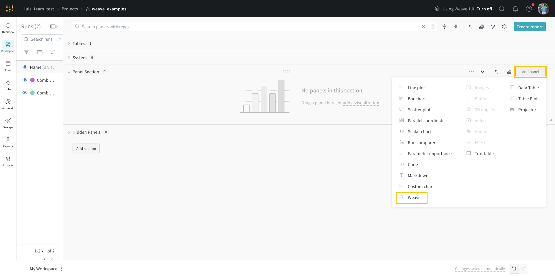
1. To add a panel globally, click Add panels in the control bar near the panel search field.
2. To add a panel directly to a section instead, click the section’s action ... menu, then click + Add panels.
3. Select the type of panel to add, such as a chart. The panel’s configuration details appear, with defaults selected.
4. Optionally, customize the panel and its display preferences. Configuration options depend on the type of panel you select. To learn more about the options for each type of panel, refer to the relevant section below, such as Line plots or Bar plots.
5. Click Apply.

Quick add panels

Use Quick add to add a panel automatically for each key you select, either globally or at the section level.

For an automated workspace with no deleted panels, the Quick add option is not visible because the workspace already includes panels for all logged keys. You can use Quick add to re-add a panel that you deleted.

1. To use Quick add to add a panel globally, click Add panels in the control bar near the panel search field, then click Quick add.
2. To use Quick add to add a panel directly to a section, click the section’s action ... menu, click Add panels, then click Quick add.
3. A list of panels appears. Each panel with a checkmark is already included in the workspace.
   • To add all available panels, click the Add panels button at the top of the list. The Quick Add list closes and the new panels display in the workspace.
   • To add an individual panel from the list, hover over the panel’s row, then click Add. Repeat this step for each panel you want to add, then click the X at the top right to close the Quick Add list. The new panels display in the workspace.
4. Optionally, customize the panel’s settings.

Share a panel

This section shows how to share a panel using a link.

To share a panel using a link, you can either:

• While viewing the panel in full-screen mode, copy the URL from the browser.
• Click the action menu ... and select Copy panel URL.

Share the link with the user or team. When they access the link, the panel opens in full-screen mode.

To return to a panel’s workspace from full-screen mode, click the left-pointing arrow at the top of the page.

Compose a panel’s full-screen link programmatically

In certain situations, such as when creating an automation, it can be useful to include the panel’s full-screen URL. This section shows the format for a panel’s full-screen URL. In the proceeding example, replace the entity, project, panel, and section names in brackets.

https://wandb.ai/<ENTITY_NAME>/<PROJECT_NAME>?panelDisplayName=<PANEL_NAME>&panelSectionName=<SECTON_NAME>

If multiple panels in the same section have the same name, this URL opens the first panel with the name.

Embed or share a panel on social media

To embed a panel in a website or share it on social media, the panel must be viewable by anyone with the link. If a project is private, only members of the project can view the panel. If the project is public, anyone with the link can view the panel.

To get the code to embed or share a panel on social media:

1. From the workspace, hover over the panel, then click its action menu ....
2. Click the Share tab.
3. Change Only those who are invited have access to Anyone with the link can view. Otherwise, the choices in the next step are not available.
4. Choose Share on Twitter, Share on Reddit, Share on LinkedIn, or Copy embed link.

Email a panel report

To email a single panel as a stand-alone report:

1. Hover over the panel, then click the panel’s action menu ....
2. Click Share panel in report.
3. Select the Invite tab.
4. Enter an email address or username.
5. Optionally, change can view to can edit.
6. Click Invite. W&B sends an email to the user with a clickable link to the report that contains only the panel you are sharing.

Unlike when you share a panel, the recipient cannot get to the workspace from this report.

Manage panels

Edit a panel

To edit a panel:

1. Click its pencil icon.
2. Modify the panel’s settings.
3. To change the panel to a different type, select the type and then configure the settings.
4. Click Apply.

Move a panel

To move a panel to a different section, you can use the drag handle on the panel. To select the new section from a list instead:

1. If necessary, create a new section by clicking Add section after the last section.
2. Click the action ... menu for the panel.
3. Click Move, then select a new section.

You can also use the drag handle to rearrange panels within a section.

Duplicate a panel

To duplicate a panel:

1. At the top of the panel, click the action ... menu.
2. Click Duplicate.

If desired, you can customize or move the duplicated panel.

Remove panels

To remove a panel:

1. Hover your mouse over the panel.
2. Select the action ... menu.
3. Click Delete.

To remove all panels from a manual workspace, click its action ... menu, then click Clear all panels.

To remove all panels from an automatic or manual workspace, you can reset the workspace. Select Automatic to start with the default set of panels, or select Manual to start with an empty workspace with no panels.

Manage sections

By default, sections in a workspace reflect the logging hierarchy of your keys. However, in a manual workspace, sections appear only after you start adding panels.

Add a section

To add a section, click Add section after the last section.

To add a new section before or after an existing section, you can instead click the section’s action ... menu, then click New section below or New section above.

Manage a section’s panels

Sections with a large number of panels are paginated by default if they use the Standard grid layout. The default number of panels on a page depend on the panel’s configuration and on the sizes of the panels in the section.

1. To check which layout a section uses, click the section’s action ... menu. To change a section’s layout, select Standard grid or Custom grid in the Layout grid section.
2. To resize a panel, hover over it, click the drag handle, and drag it to adjust the panel’s size.

• If a section uses the Standard grid, resizing one panel resizes all panels in the section.
• If a section uses the Custom grid, you can customize the size of each panel separately.

1. If a section is paginated, you can customize the number of panels to show on a page:
2. At the top of the section, click 1 to of , where <X> is the number of visible panels and <Y> is the total number of panels.
3. Choose how many panels to show per page, up to 100.
4. To show all panels when there are a large number of them, configure the panel to use the Custom grid layout. Click the section’s action ... menu, then select Custom grid in the Layout grid section
5. To delete a panel from a section:
6. Hover over the panel, then click its action ... menu.
7. Click Delete.

If you reset a workspace to an automated workspace, all deleted panels appear again.

Rename a section

To rename a section, click its action ... menu, then click Rename section.

Delete a section

To delete a section, click its ... menu, then click Delete section. This removes the section and its panels.

1 - Line plots

Line plots show up by default when you plot metrics over time with wandb.log(). Customize with chart settings to compare multiple lines on the same plot, calculate custom axes, and rename labels.

Edit line plot settings

This section shows how to edit the settings for an individual line plot panel, all line plot panels in a section, or all line plot panels in a workspace.

Individual line plot

A line plot’s individual settings override the line plot settings for the section or the workspace. To customize a line plot:

1. Hover your mouse over the panel, then click the gear icon.
2. Within the modal that appears, select a tab to edit its settings.
3. Click Apply.

Line plot settings

You can configure these settings for a line plot:

Date: Configure the plot’s data-display details.

• X: Select the value to use for the X axis (defaults to Step). You can change the x-axis to Relative Time or select a custom axis based on values you log with W&B.
  • Relative Time (Wall) is clock time since the process started, so if you started a run and resumed it a day later and logged something that would be plotted a 24hrs.
  • Relative Time (Process) is time inside the running process, so if you started a run and ran for 10 seconds and resumed a day later that point would be plotted at 10s.
  • Wall Time is minutes elapsed since the start of the first run on the graph.
  • Step increments by default each time wandb.log() is called, and is supposed to reflect the number of training steps you’ve logged from your model.
• Y: Select one or more y-axes from the logged values, including metrics and hyperparameters that change over time.
• X Axis and Y Axis minimum and maximum values (optional).
• Point aggregation method. Either Random sampling (the default) or Full fidelity. Refer to Sampling.
• Smoothing: Change the smoothing on the line plot. Defaults to Time weighted EMA. Other values include No smoothing, Running average, and Gaussian.
• Outliers: Rescale to exclude outliers from the default plot min and max scale.
• Max number of runs or groups: Show more lines on the line plot at once by increasing this number, which defaults to 10 runs. You’ll see the message “Showing first 10 runs” on the top of the chart if there are more than 10 runs available but the chart is constraining the number visible.
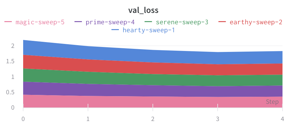
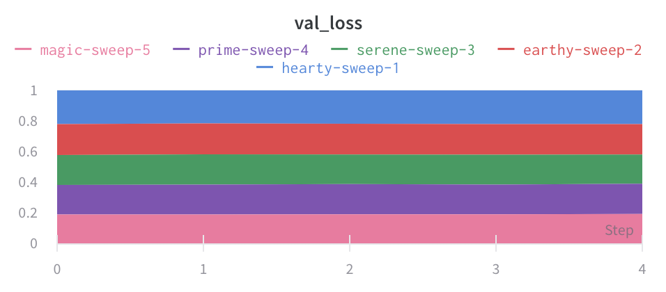
• Chart type: Change between a line plot, an area plot, and a percentage area plot.

Grouping: Configure whether and how to group and aggregate runs in the plot.

• Group by: Select a column, and all the runs with the same value in that column will be grouped together.
• Agg: Aggregation— the value of the line on the graph. The options are mean, median, min, and max of the group.

Chart: Specify titles for the panel, the X axis, and the Y axis, and the -axis, hide or show the legend, and configure its position.

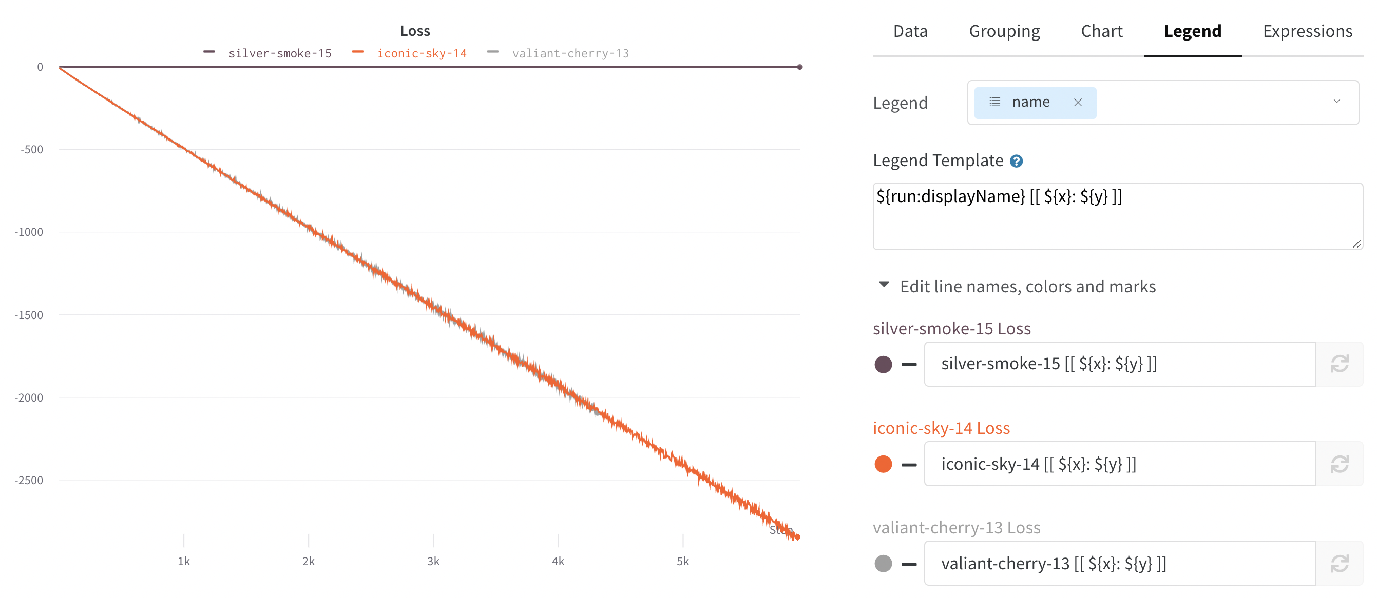
Legend: Customize the appearance of the panel’s legend, if it is enabled.

• Legend: The field in the legend for each line in the plot in the legend of the plot for each line.
• Legend template: Define a fully customizable template for the legend, specifying exactly what text and variables you want to show up in the template at the top of the line plot as well as the legend that appears when you hover your mouse over the plot.

Expressions: Add custom calculated expressions to the panel.

• Y Axis Expressions: Add calculated metrics to your graph. You can use any of the logged metrics as well as configuration values like hyperparameters to calculate custom lines.
• X Axis Expressions: Rescale the x-axis to use calculated values using custom expressions. Useful variables include**_step** for the default x-axis, and the syntax for referencing summary values is ${summary:value}

All line plots in a section

To customize the default settings for all line plots in a section, overriding workspace settings for line plots:

1. Click the section’s gear icon to open its settings.
2. Within the modal that appears, select the Data or Display preferences tabs to configure the default settings for the section. For details about each Data setting, refer to the preceding section, Individual line plot. For details about each display preference, refer to Configure section layout.

All line plots in a workspace

To customize the default settings for all line plots in a workspace:

1. Click the workspace’s settings, which has a gear with the label Settings.
2. Click Line plots.
3. Within the modal that appears, select the Data or Display preferences tabs to configure the default settings for the workspace.

   • For details about each Data setting, refer to the preceding section, Individual line plot.

   • For details about each Display preferences section, refer to Workspace display preferences. At the workspace level, you can configure the default Zooming behavior for line plots. This setting controls whether to synchronize zooming across line plots with a matching x-axis key. Disabled by default.

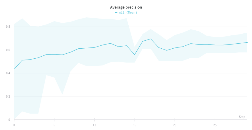
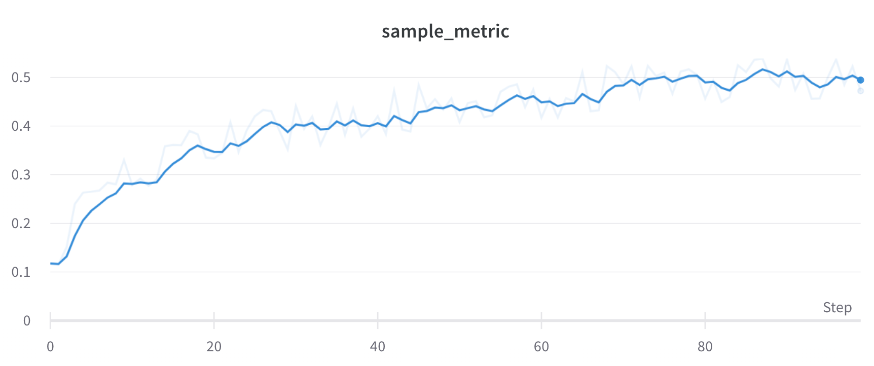
Visualize average values on a plot

If you have several different experiments and you’d like to see the average of their values on a plot, you can use the Grouping feature in the table. Click “Group” above the run table and select “All” to show averaged values in your graphs.

Here is what the graph looks like before averaging:

The proceeding image shows a graph that represents average values across runs using grouped lines.

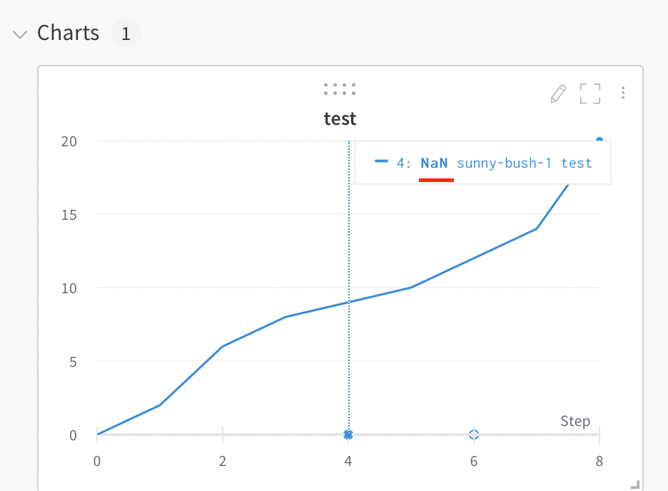
Visualize NaN value on a plot

You can also plot NaN values including PyTorch tensors on a line plot with wandb.log. For example:

wandb.log({"test": [..., float("nan"), ...]})

Compare two metrics on one chart

1. Select the Add panels button in the top right corner of the page.
2. From the left panel that appears, expand the Evaluation dropdown.
3. Select Run comparer

Change the color of the line plots

Sometimes the default color of runs is not helpful for comparison. To help overcome this, wandb provides two instances with which one can manually change the colors.

• From the run table
• From the chart legend settings

Each run is given a random color by default upon initialization.

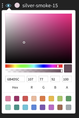
Upon clicking any of the colors, a color palette appears from which we can manually choose the color we want.

1. Hover your mouse over the panel you want to edit its settings for.
2. Select the pencil icon that appears.
3. Choose the Legend tab.

Visualize on different x axes

If you’d like to see the absolute time that an experiment has taken, or see what day an experiment ran, you can switch the x axis. Here’s an example of switching from steps to relative time and then to wall time.

Area plots

In the line plot settings, in the advanced tab, click on different plot styles to get an area plot or a percentage area plot.

Zoom

Click and drag a rectangle to zoom vertically and horizontally at the same time. This changes the x-axis and y-axis zoom.

Hide chart legend

Turn off the legend in the line plot with this simple toggle:

1.1 - Line plot reference

X-Axis

You can set the x-axis of a line plot to any value that you have logged with W&B.log as long as it’s always logged as a number.

Y-Axis variables

You can set the y-axis variables to any value you have logged with wandb.log as long as you were logging numbers, arrays of numbers or a histogram of numbers. If you logged more than 1500 points for a variable, W&B samples down to 1500 points.

X range and Y range

You can change the maximum and minimum values of X and Y for the plot.

X range default is from the smallest value of your x-axis to the largest.

Y range default is from the smallest value of your metrics and zero to the largest value of your metrics.

Max runs/groups

By default you will only plot 10 runs or groups of runs. The runs will be taken from the top of your runs table or run set, so if you sort your runs table or run set you can change the runs that are shown.

Legend

You can control the legend of your chart to show for any run any config value that you logged and meta data from the runs such as the created at time or the user who created the run.

Example:

${run:displayName} - ${config:dropout} will make the legend name for each run something like royal-sweep - 0.5 where royal-sweep is the run name and 0.5 is the config parameter named dropout.

You can set value inside[[ ]] to display point specific values in the crosshair when hovering over a chart. For example \[\[ $x: $y ($original) ]] would display something like “2: 3 (2.9)”

Supported values inside [[ ]] are as follows:

Grouping

You can aggregate all of the runs by turning on grouping, or group over an individual variable. You can also turn on grouping by grouping inside the table and the groups will automatically populate into the graph.

Smoothing

You can set the smoothing coefficient to be between 0 and 1 where 0 is no smoothing and 1 is maximum smoothing.

Ignore outliers

Rescale the plot to exclude outliers from the default plot min and max scale. The setting’s impact on the plot depends on the plot’s sampling mode.

• For plots that use random sampling mode, when you enable Ignore outliers, only points from 5% to 95% are shown. When outliers are shown, they are not formatted differently from other points.
• For plots that use full fidelity mode, all points are always shown, condensed down to the last value in each bucket. When Ignore outliers is enabled, the minimum and maximum bounds of each bucket are shaded. Otherwise, no area is shaded.

Expression

Expression lets you plot values derived from metrics like 1-accuracy. It currently only works if you are plotting a single metric. You can do simple arithmetic expressions, +, -, *, / and % as well as ** for powers.

Plot style

Select a style for your line plot.

Line plot:

Area plot:

Percentage area plot:

1.2 - Point aggregation

Use point aggregation methods within your line plots for improved data visualization accuracy and performance. There are two types of point aggregation modes: full fidelity and random sampling. W&B uses full fidelity mode by default.

Full fidelity

When you use full fidelity mode, W&B breaks the x-axis into dynamic buckets based on the number of data points. It then calculates the minimum, maximum, and average values within each bucket while rendering a point aggregation for the line plot.

There are three main advantages to using full fidelity mode for point aggregation:

• Preserve extreme values and spikes: retain extreme values and spikes in your data
• Configure how minimum and maximum points render: use the W&B App to interactively decide whether you want to show extreme (min/max) values as a shaded area.
• Explore your data without losing data fidelity: W&B recalculates x-axis bucket sizes when you zoom into specific data points. This helps ensure that you can explore your data without losing accuracy. Caching is used to store previously computed aggregations to help reduce loading times which is particularly useful if you are navigating through large datasets.

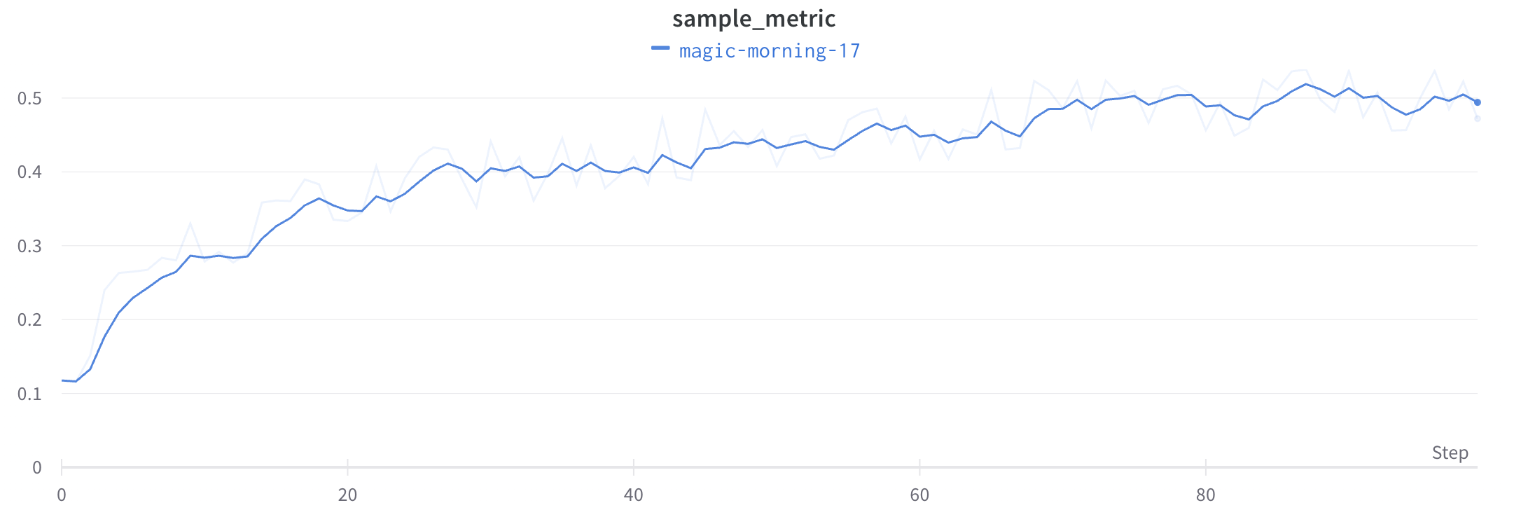
Configure how minimum and maximum points render

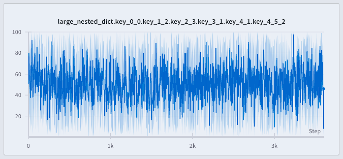
Show or hide minimum and maximum values with shaded areas around your line plots.

The proceeding image shows a blue line plot. The light blue shaded area represents the minimum and maximum values for each bucket.

There are three ways to render minimum and maximum values in your line plots:

• Never: The min/max values are not displayed as a shaded area. Only show the aggregated line across the x-axis bucket.
• On hover: The shaded area for min/max values appears dynamically when you hover over the chart. This option keeps the view uncluttered while allowing you to inspect ranges interactively.
• Always: The min/max shaded area is consistently displayed for every bucket in the chart, helping you visualize the full range of values at all times. This can introduce visual noise if there are many runs visualized in the chart.

By default, the minimum and maximum values are not displayed as shaded areas. To view one of the shaded area options, follow these steps:

• All charts in a workspace
• Individual chart in a workspace

Explore your data without losing data fidelity

Analyze specific regions of the dataset without missing critical points like extreme values or spikes. When you zoom in on a line plot, W&B adjusts the buckets sizes used to calculate the minimum, maximum, and average values within each bucket.

W&B divides the x-axis is dynamically into 1000 buckets by default. For each bucket, W&B calculates the following values:

• Minimum: The lowest value in that bucket.
• Maximum: The highest value in that bucket.
• Average: The mean value of all points in that bucket.

W&B plots values in buckets in a way that preserves full data representation and includes extreme values in every plot. When zoomed in to 1,000 points or fewer, full fidelity mode renders every data point without additional aggregation.

To zoom in on a line plot, follow these steps:

1. Navigate to your W&B project
2. Select on the Workspace icon on the left tab
3. Optionally add a line plot panel to your workspace or navigate to an existing line plot panel.
4. Click and drag to select a specific region to zoom in on.

Random sampling

Random sampling uses 1500 randomly sampled points to render line plots. Random sampling is useful for performance reasons when you have a large number of data points.

Enable random sampling

By default, W&B uses full fidelity mode. To enable random sampling, follow these steps:

• All charts in a workspace
• Individual chart in a workspace

Access non sampled data

You can access the complete history of metrics logged during a run using the W&B Run API. The following example demonstrates how to retrieve and process the loss values from a specific run:

# Initialize the W&B API
run = api.run("l2k2/examples-numpy-boston/i0wt6xua")

# Retrieve the history of the 'Loss' metric
history = run.scan_history(keys=["Loss"])

# Extract the loss values from the history
losses = [row["Loss"] for row in history]

1.3 - Smooth line plots

W&B supports three types of smoothing:

• exponential moving average (default)
• gaussian smoothing
• running average
• exponential moving average - Tensorboard (deprecated)

See these live in an interactive W&B report.

Exponential Moving Average (Default)

Exponential smoothing is a technique for smoothing time series data by exponentially decaying the weight of previous points. The range is 0 to 1. See Exponential Smoothing for background. There is a de-bias term added so that early values in the time series are not biased towards zero.

The EMA algorithm takes the density of points on the line (the number of y values per unit of range on x-axis) into account. This allows consistent smoothing when displaying multiple lines with different characteristics simultaneously.

Here is sample code for how this works under the hood:

const smoothingWeight = Math.min(Math.sqrt(smoothingParam || 0), 0.999);
let lastY = yValues.length > 0 ? 0 : NaN;
let debiasWeight = 0;

return yValues.map((yPoint, index) => {
  const prevX = index > 0 ? index - 1 : 0;
  // VIEWPORT_SCALE scales the result to the chart's x-axis range
  const changeInX =
    ((xValues[index] - xValues[prevX]) / rangeOfX) * VIEWPORT_SCALE;
  const smoothingWeightAdj = Math.pow(smoothingWeight, changeInX);

  lastY = lastY * smoothingWeightAdj + yPoint;
  debiasWeight = debiasWeight * smoothingWeightAdj + 1;
  return lastY / debiasWeight;
});

Here’s what this looks like in the app:

Gaussian Smoothing

Gaussian smoothing (or gaussian kernel smoothing) computes a weighted average of the points, where the weights correspond to a gaussian distribution with the standard deviation specified as the smoothing parameter. See . The smoothed value is calculated for every input x value.

Gaussian smoothing is a good standard choice for smoothing if you are not concerned with matching TensorBoard’s behavior. Unlike an exponential moving average the point will be smoothed based on points occurring both before and after the value.

Here’s what this looks like in the app:

Running Average

Running average is a smoothing algorithm that replaces a point with the average of points in a window before and after the given x value. See “Boxcar Filter” at https://en.wikipedia.org/wiki/Moving_average. The selected parameter for running average tells Weights and Biases the number of points to consider in the moving average.

Consider using Gaussian Smoothing if your points are spaced unevenly on the x-axis.

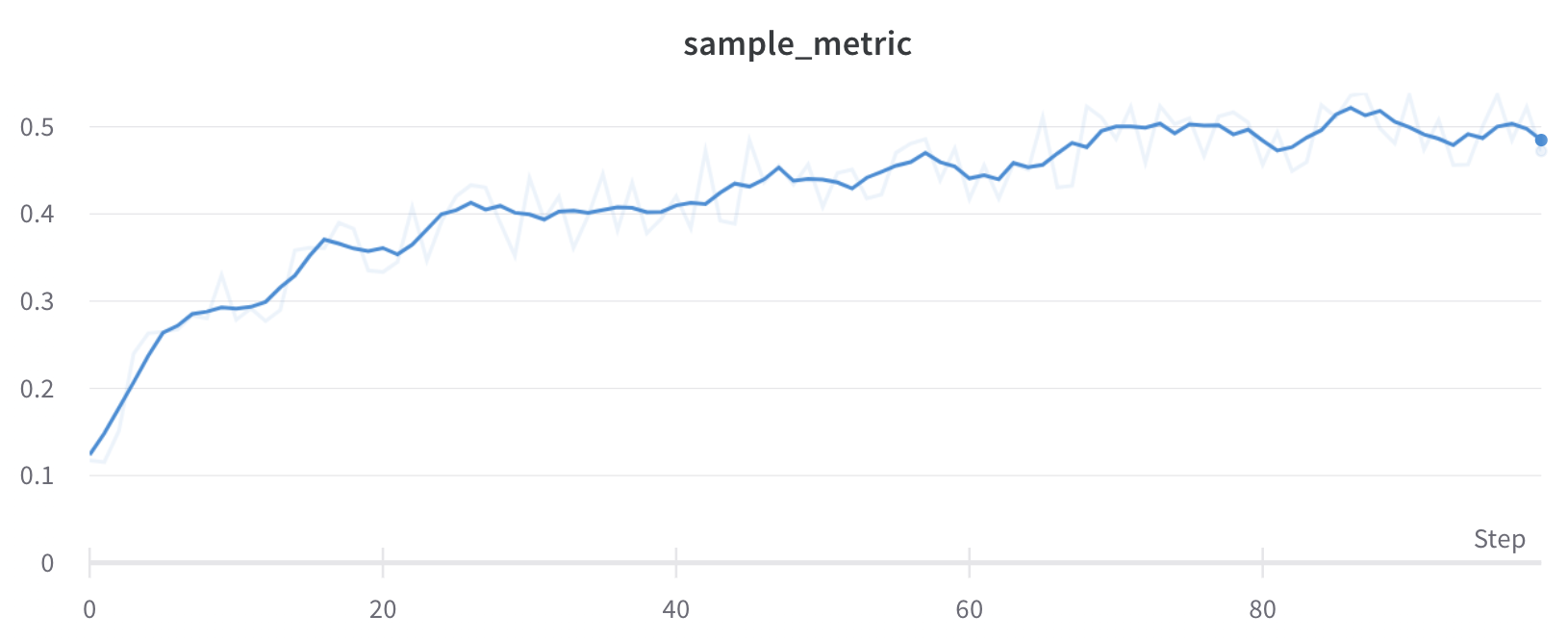
The following image demonstrates how a running app looks like in the app:

Exponential Moving Average (Deprecated)

The TensorBoard EMA algorithm has been deprecated as it cannot accurately smooth multiple lines on the same chart that do not have a consistent point density (number of points plotted per unit of x-axis).

Exponential moving average is implemented to match TensorBoard’s smoothing algorithm. The range is 0 to 1. See Exponential Smoothing for background. There is a debias term added so that early values in the time series are not biases towards zero.

Here is sample code for how this works under the hood:

  data.forEach(d => {
    const nextVal = d;
    last = last * smoothingWeight + (1 - smoothingWeight) * nextVal;
    numAccum++;
    debiasWeight = 1.0 - Math.pow(smoothingWeight, numAccum);
    smoothedData.push(last / debiasWeight);

Here’s what this looks like in the app:

Implementation Details

All of the smoothing algorithms run on the sampled data, meaning that if you log more than 1500 points, the smoothing algorithm will run after the points are downloaded from the server. The intention of the smoothing algorithms is to help find patterns in data quickly. If you need exact smoothed values on metrics with a large number of logged points, it may be better to download your metrics through the API and run your own smoothing methods.

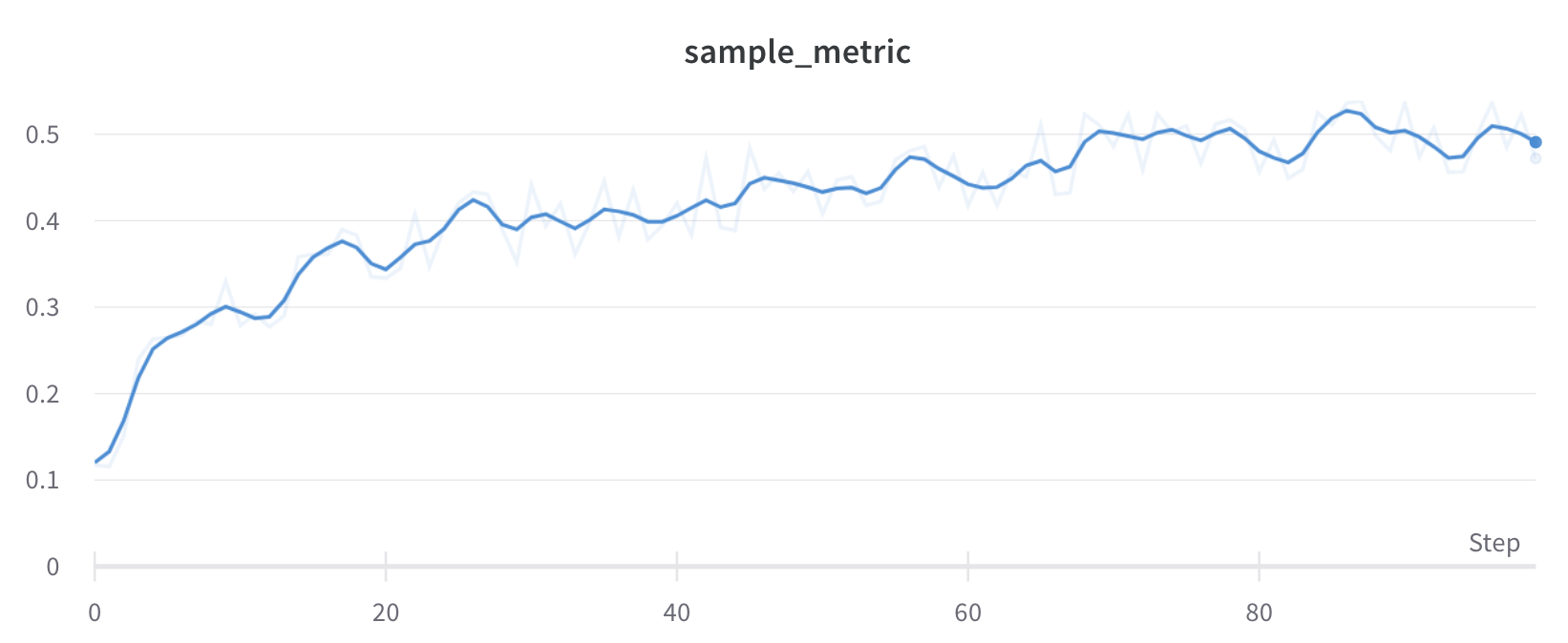
Hide original data

By default we show the original, unsmoothed data as a faint line in the background. Click the Show Original toggle to turn this off.

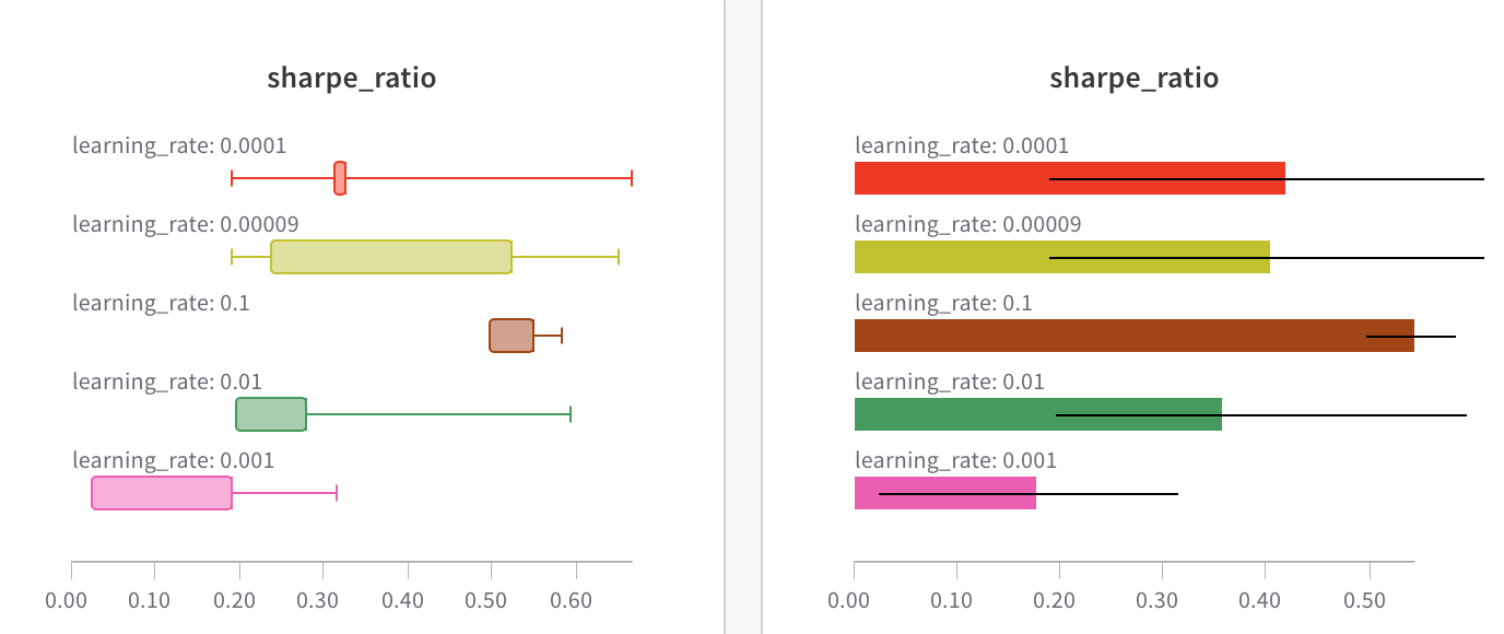
2 - Bar plots

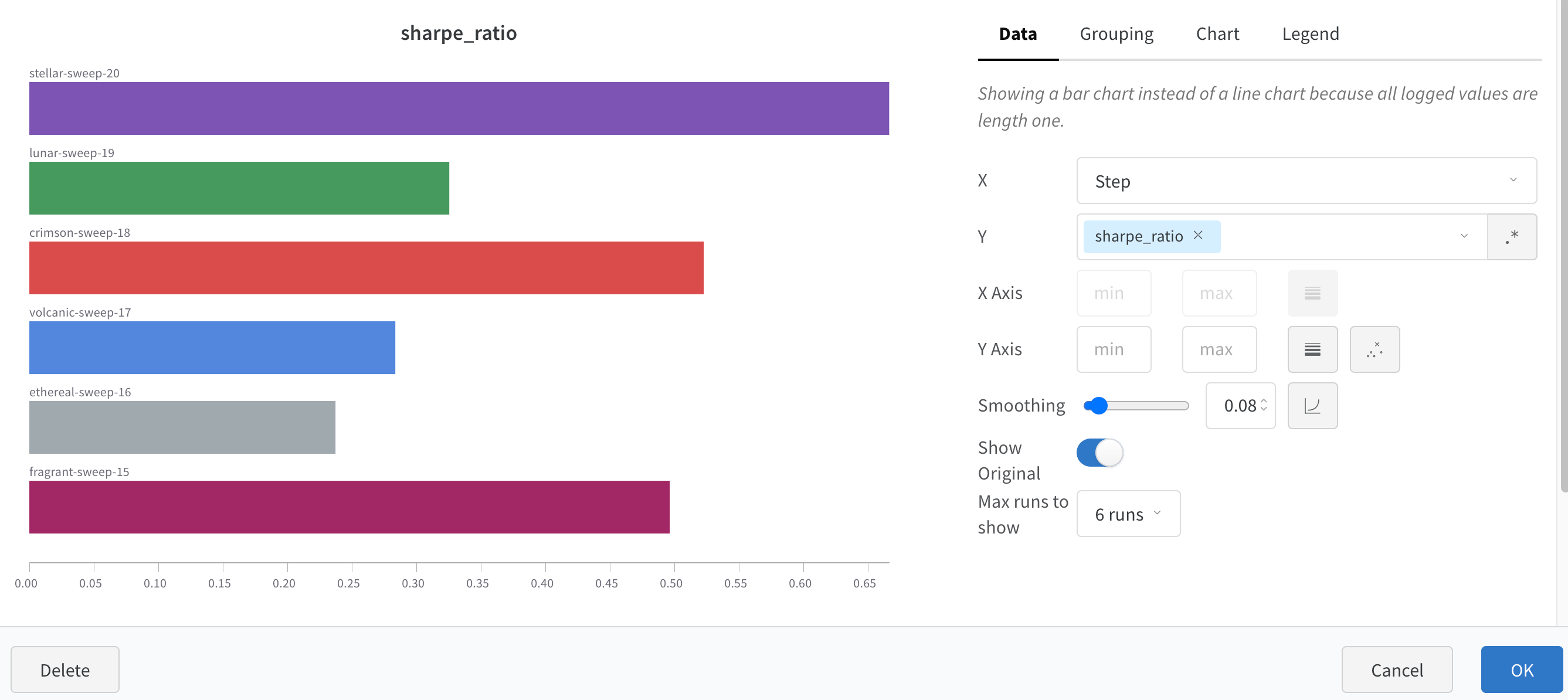
A bar plot presents categorical data with rectangular bars which can be plotted vertically or horizontally. Bar plots show up by default with wandb.log() when all logged values are of length one.

Customize with chart settings to limit max runs to show, group runs by any config and rename labels.

Customize bar plots

You can also create Box or Violin Plots to combine many summary statistics into one chart type**.**

1. Group runs via runs table.
2. Click ‘Add panel’ in the workspace.
3. Add a standard ‘Bar Chart’ and select the metric to plot.
4. Under the ‘Grouping’ tab, pick ‘box plot’ or ‘Violin’, etc. to plot either of these styles.

3 - Parallel coordinates

Parallel coordinates charts summarize the relationship between large numbers of hyperparameters and model metrics at a glance.

• Axes: Different hyperparameters from wandb.config and metrics from wandb.log.
• Lines: Each line represents a single run. Mouse over a line to see a tooltip with details about the run. All lines that match the current filters will be shown, but if you turn off the eye, lines will be grayed out.

Create a parallel coordinates panel

1. Go to the landing page for your workspace
2. Click Add Panels
3. Select Parallel coordinates

Panel Settings

To configure the panel, click the edit button in the upper right corner of the panel.

• Tooltip: On hover, a legend shows up with info on each run
• Titles: Edit the axis titles to be more readable
• Gradient: Customize the gradient to be any color range you like
• Log scale: Each axis can be set to view on a log scale independently
• Flip axis: Switch the axis direction— this is useful when you have both accuracy and loss as columns

Interact with a live parallel coordinates panel

4 - Scatter plots

This page shows how to use scatter plots in W&B.

Use case

Use scatter plots to compare multiple runs and visualize the performance of an experiment:

• Plot lines for minimum, maximum, and average values.
• Customize metadata tooltips.
• Control point colors.
• Adjust axis ranges.
• Use a log scale for the axes.

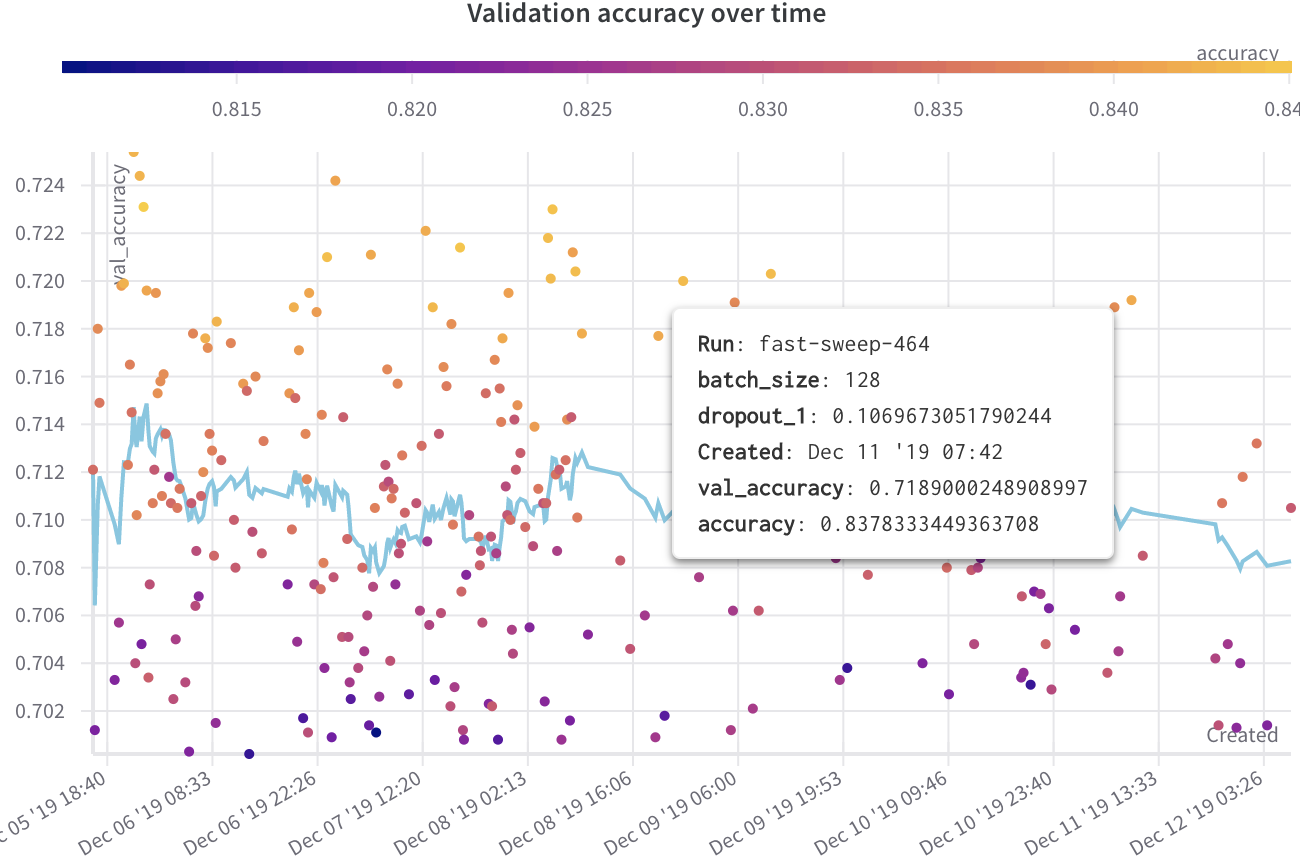
Example

The following example shows a scatter plot displaying validation accuracy for different models over several weeks of experimentation. The tooltip includes batch size, dropout, and axis values. A line also shows the running average of validation accuracy.

See a live example →

Create a scatter plot

To create a scatter plot in the W&B UI:

1. Navigate to the Workspaces tab.
2. In the Charts panel, click the action menu ....
3. From the pop-up menu, select Add panels.
4. In the Add panels menu, select Scatter plot.
5. Set the x and y axes to plot the data you want to view. Optionally, set maximum and minimum ranges for your axes or add a z axis.
6. Click Apply to create the scatter plot.
7. View the new scatter plot in the Charts panel.

5 - Save and diff code

By default, W&B only saves the latest git commit hash. You can turn on more code features to compare the code between your experiments dynamically in the UI.

Starting with wandb version 0.8.28, W&B can save the code from your main training file where you call wandb.init().

Save library code

When you enable code saving, W&B saves the code from the file that called wandb.init(). To save additional library code, you have three options:

Call wandb.run.log_code(".") after calling wandb.init()

import wandb

wandb.init()
wandb.run.log_code(".")

Pass a settings object to wandb.init with code_dir set

import wandb

wandb.init(settings=wandb.Settings(code_dir="."))

This captures all python source code files in the current directory and all subdirectories as an artifact. For more control over the types and locations of source code files that are saved, see the reference docs.

Set code saving in the UI

In addition to setting code saving programmatically, you can also toggle this feature in your W&B account Settings. Note that this will enable code saving for all teams associated with your account.

By default, W&B disables code saving for all teams.

1. Log in to your W&B account.
2. Go to Settings > Privacy.
3. Under Project and content security, toggle Disable default code saving on.

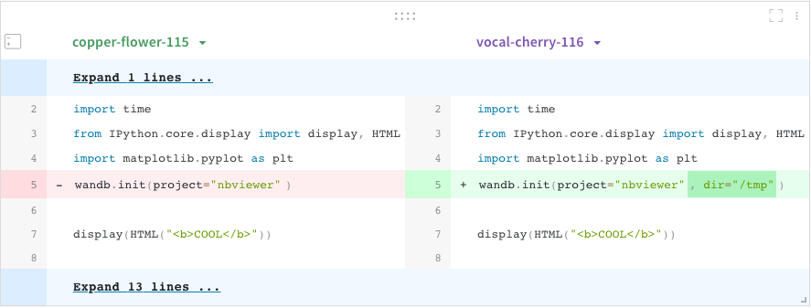
Code comparer

Compare code used in different W&B runs:

1. Select the Add panels button in the top right corner of the page.
2. Expand TEXT AND CODE dropdown and select Code.

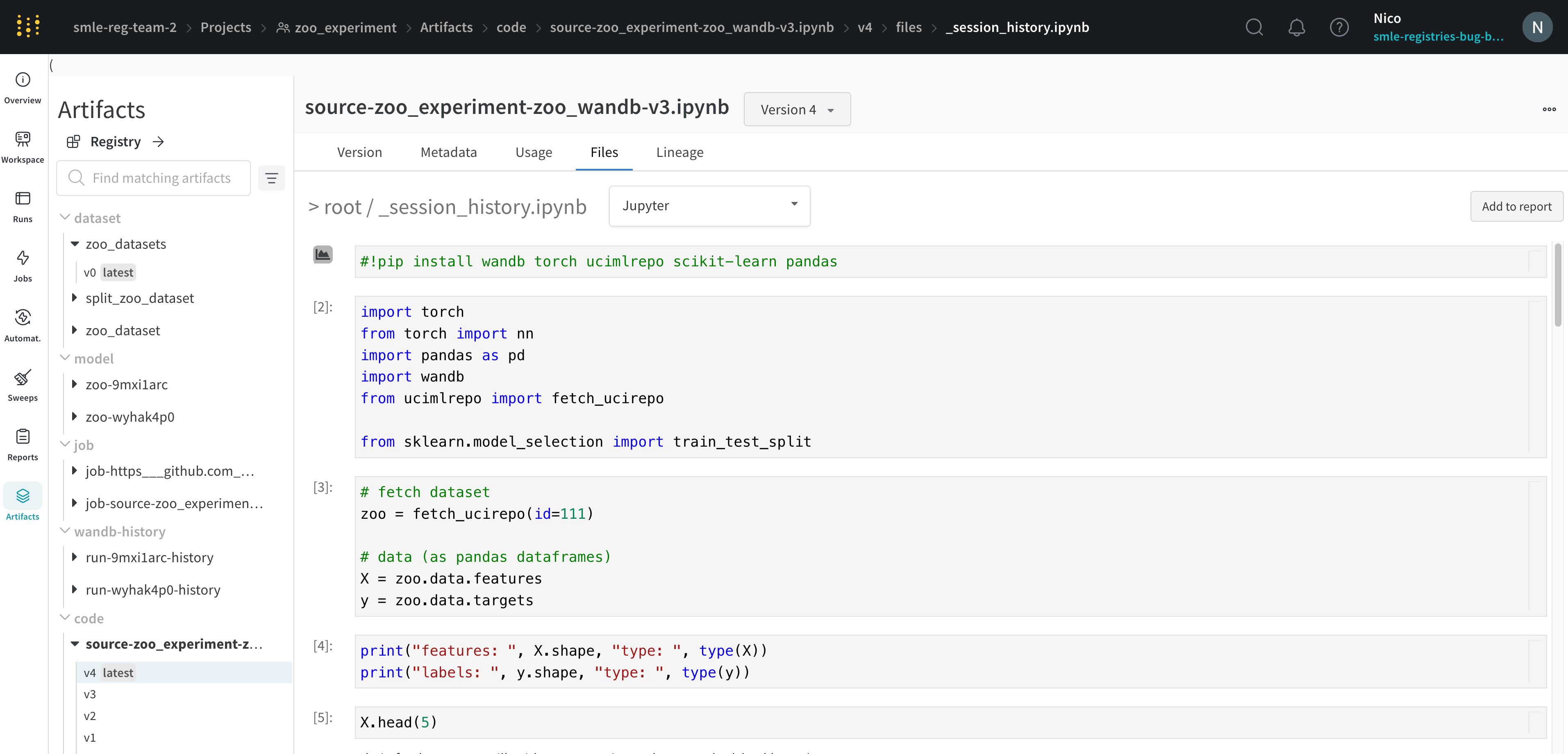
Jupyter session history

W&B saves the history of code executed in your Jupyter notebook session. When you call wandb.init() inside of Jupyter, W&B adds a hook to automatically save a Jupyter notebook containing the history of code executed in your current session.

1. Navigate to your project workspaces that contains your code.
2. Select the Artifacts tab in the left navigation bar.
3. Expand the code artifact.
4. Select the Files tab.

This displays the cells that were run in your session along with any outputs created by calling iPython’s display method. This enables you to see exactly what code was run within Jupyter in a given run. When possible W&B also saves the most recent version of the notebook which you would find in the code directory as well.

6 - Parameter importance

Discover which of your hyperparameters were the best predictors of, and highly correlated to desirable values of your metrics.

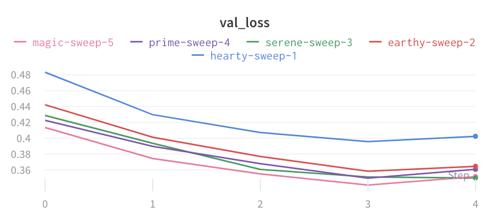
Correlation is the linear correlation between the hyperparameter and the chosen metric (in this case val_loss). So a high correlation means that when the hyperparameter has a higher value, the metric also has higher values and vice versa. Correlation is a great metric to look at but it can’t capture second order interactions between inputs and it can get messy to compare inputs with wildly different ranges.

Therefore W&B also calculates an importance metric. W&B trains a random forest with the hyperparameters as inputs and the metric as the target output and report the feature importance values for the random forest.

The idea for this technique was inspired by a conversation with Jeremy Howard who has pioneered the use of random forest feature importances to explore hyperparameter spaces at Fast.ai. W&B highly recommends you check out this lecture (and these notes) to learn more about the motivation behind this analysis.

Hyperparameter importance panel untangles the complicated interactions between highly correlated hyperparameters. In doing so, it helps you fine tune your hyperparameter searches by showing you which of your hyperparameters matter the most in terms of predicting model performance.

Creating a hyperparameter importance panel

1. Navigate to your W&B project.
2. Select Add panels buton.
3. Expand the CHARTS dropdown, choose Parallel coordinates from the dropdown.

With the parameter manager, we can manually set the visible and hidden parameters.

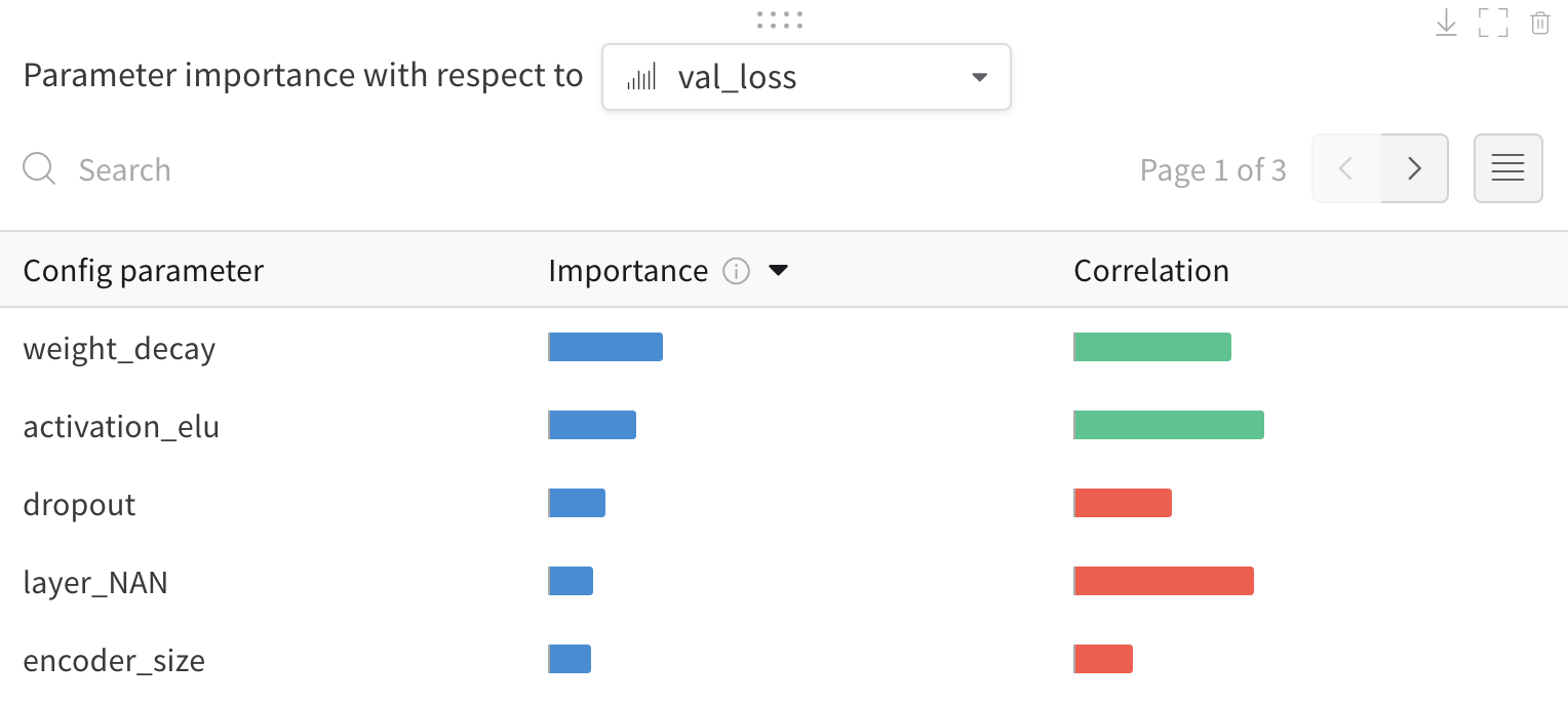
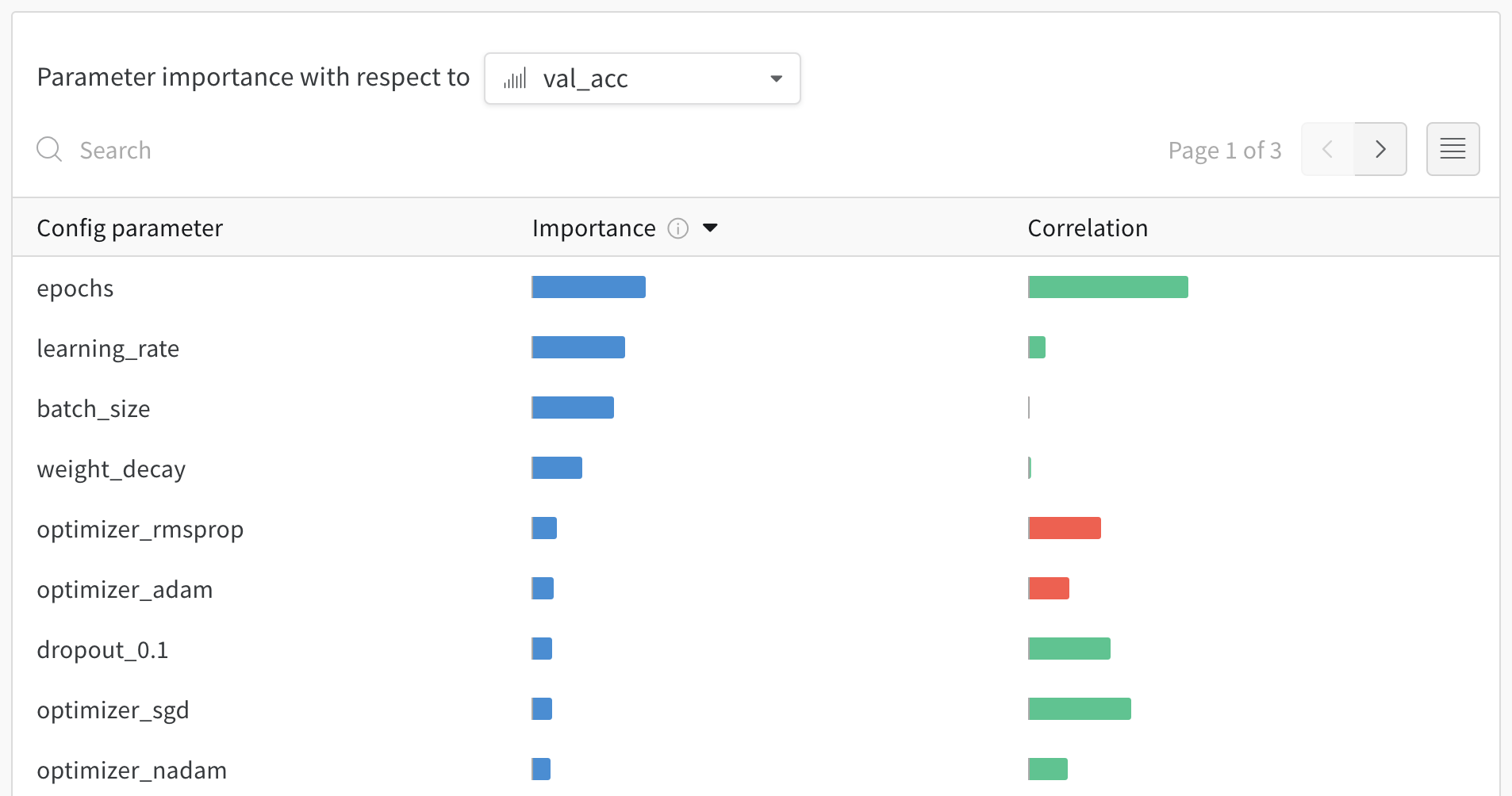
Interpreting a hyperparameter importance panel

This panel shows you all the parameters passed to the wandb.config object in your training script. Next, it shows the feature importances and correlations of these config parameters with respect to the model metric you select (val_loss in this case).

Importance

The importance column shows you the degree to which each hyperparameter was useful in predicting the chosen metric. Imagine a scenario were you start tuning a plethora of hyperparameters and using this plot to hone in on which ones merit further exploration. The subsequent sweeps can then be limited to the most important hyperparameters, thereby finding a better model faster and cheaper.

In the preceding image, you can see that epochs, learning_rate, batch_size and weight_decay were fairly important.

Correlations

Correlations capture linear relationships between individual hyperparameters and metric values. They answer the question of whether there a significant relationship between using a hyperparameter, such as the SGD optimizer, and the val_loss (the answer in this case is yes). Correlation values range from -1 to 1, where positive values represent positive linear correlation, negative values represent negative linear correlation and a value of 0 represents no correlation. Generally a value greater than 0.7 in either direction represents strong correlation.

You might use this graph to further explore the values that are have a higher correlation to our metric (in this case you might pick stochastic gradient descent or adam over rmsprop or nadam) or train for more epochs.

The disparities between importance and correlations result from the fact that importance accounts for interactions between hyperparameters, whereas correlation only measures the affects of individual hyperparameters on metric values. Secondly, correlations capture only the linear relationships, whereas importances can capture more complex ones.

As you can see both importance and correlations are powerful tools for understanding how your hyperparameters influence model performance.

7 - Compare run metrics

Use the Run Comparer to see what metrics are different across your runs.

1. Select the Add panels button in the top right corner of the page.
2. From the left panel that appears, expand the Evaluation dropdown.
3. Select Run comparer

Toggle the diff only option to hide rows where the values are the same across runs.​​

8 - Query panels

Use query panels to query and interactively visualize your data.

Create a query panel

Add a query to your workspace or within a report.

• Project workspace
• W&B Report

1. Navigate to your project’s workspace.
2. In the upper right hand corner, click Add panel.
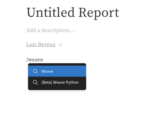
3. From the dropdown, select Query panel.

Type and select /Query panel.

Alternatively, you can associate a query with a set of runs:

1. Within your report, type and select /Panel grid.
2. Click the Add panel button.
3. From the dropdown, select Query panel.

Query components

Expressions

Use query expressions to query your data stored in W&B such as runs, artifacts, models, tables, and more.

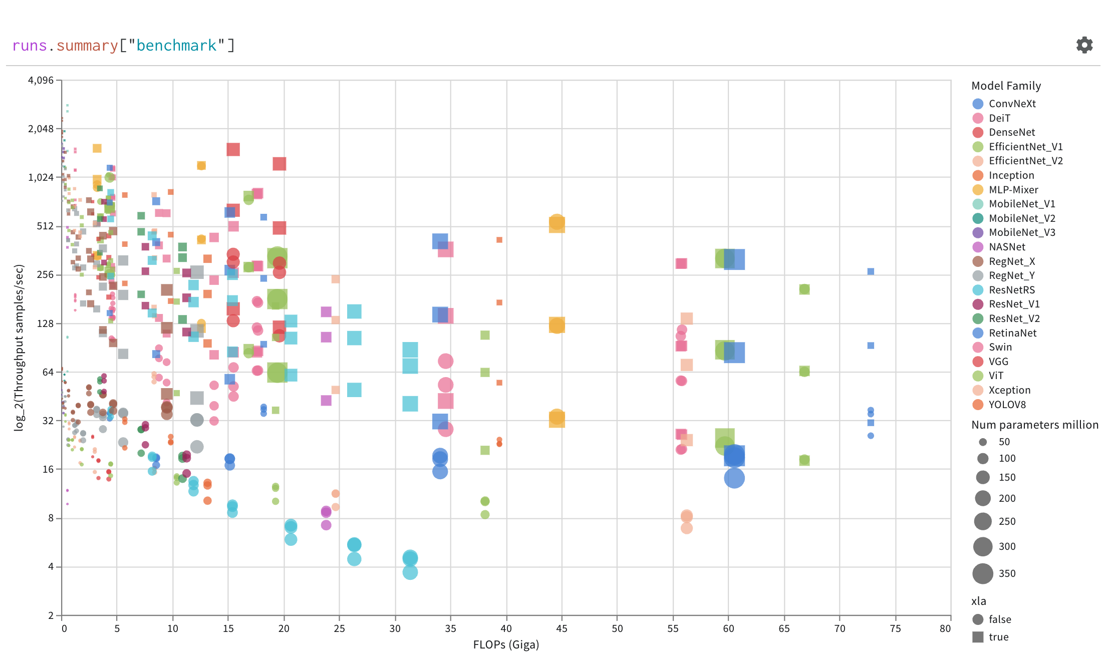
Example: Query a table

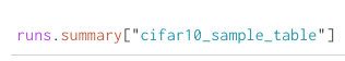
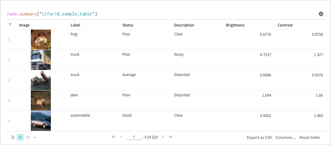
Suppose you want to query a W&B Table. In your training code you log a table called "cifar10_sample_table":

import wandb
wandb.log({"cifar10_sample_table":<MY_TABLE>})

Within the query panel you can query your table with:

runs.summary["cifar10_sample_table"]

Breaking this down:

• runs is a variable automatically injected in Query Panel Expressions when the Query Panel is in a Workspace. Its “value” is the list of runs which are visible for that particular Workspace. Read about the different attributes available within a run here.
• summary is an op which returns the Summary object for a Run. Ops are mapped, meaning this op is applied to each Run in the list, resulting in a list of Summary objects.
• ["cifar10_sample_table"] is a Pick op (denoted with brackets), with a parameter of predictions. Since Summary objects act like dictionaries or maps, this operation picks the predictions field off of each Summary object.

To learn how to write your own queries interactively, see this report.

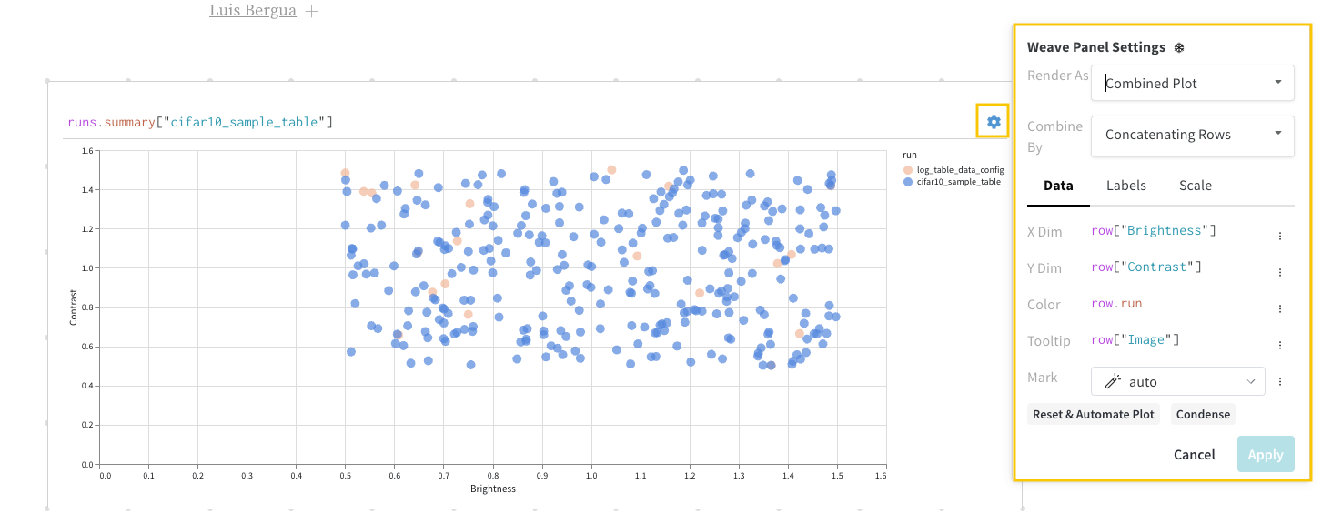
Configurations

Select the gear icon on the upper left corner of the panel to expand the query configuration. This allows the user to configure the type of panel and the parameters for the result panel.

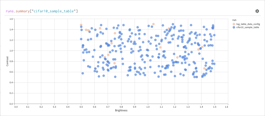
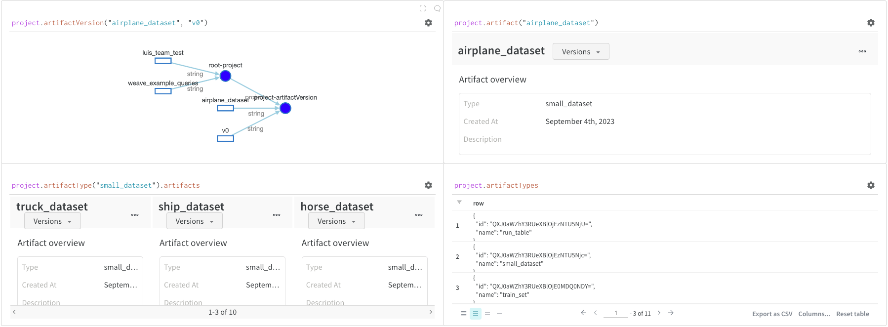
Result panels

Finally, the query result panel renders the result of the query expression, using the selected query panel, configured by the configuration to display the data in an interactive form. The following images shows a Table and a Plot of the same data.

Basic operations

The following common operations you can make within your query panels.

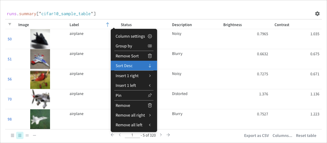
Sort

Sort from the column options:

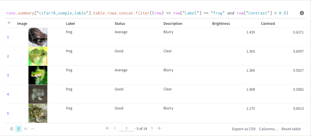
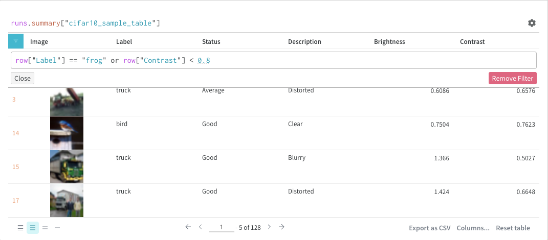
Filter

You can either filter directly in the query or using the filter button in the top left corner (second image)

Map

Map operations iterate over lists and apply a function to each element in the data. You can do this directly with a panel query or by inserting a new column from the column options.

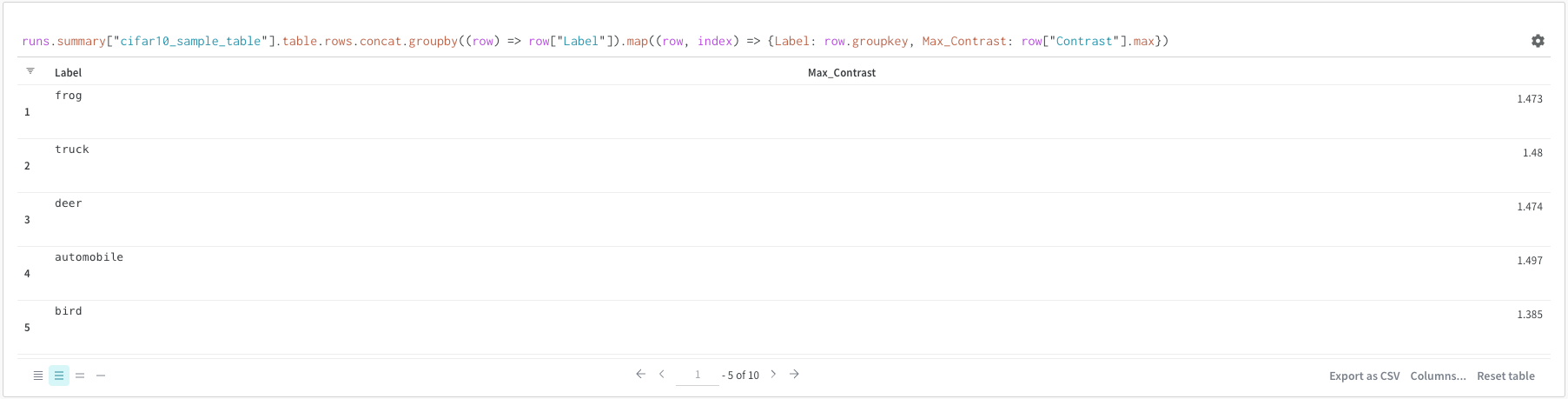
Groupby

You can groupby using a query or from the column options.

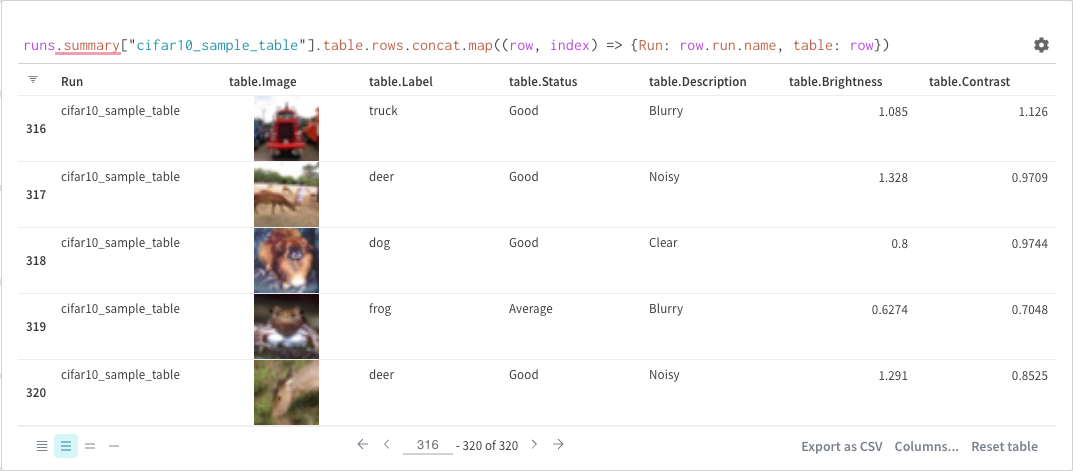
Concat

The concat operation allows you to concatenate 2 tables and concatenate or join from the panel settings

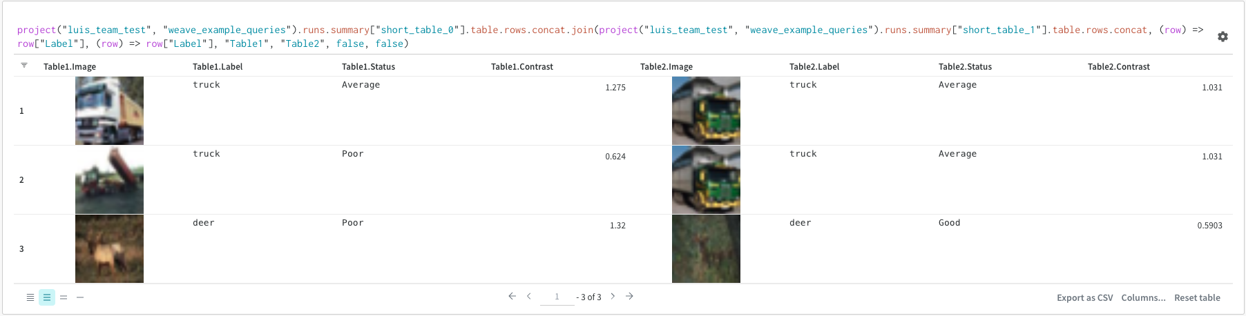
Join

It is also possible to join tables directly in the query. Consider the following query expression:

project("luis_team_test", "weave_example_queries").runs.summary["short_table_0"].table.rows.concat.join(\
project("luis_team_test", "weave_example_queries").runs.summary["short_table_1"].table.rows.concat,\
(row) => row["Label"],(row) => row["Label"], "Table1", "Table2",\
"false", "false")

The table on the left is generated from:

project("luis_team_test", "weave_example_queries").\
runs.summary["short_table_0"].table.rows.concat.join

The table in the right is generated from:

project("luis_team_test", "weave_example_queries").\
runs.summary["short_table_1"].table.rows.concat

Where:

• (row) => row["Label"] are selectors for each table, determining which column to join on
• "Table1" and "Table2" are the names of each table when joined
• true and false are for left and right inner/outer join settings

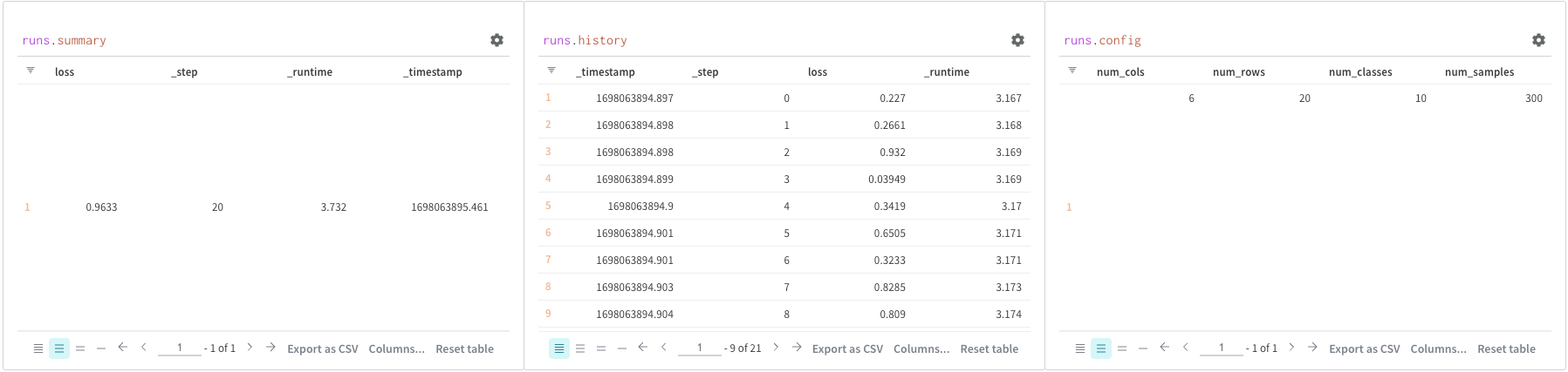
Runs object

Use query panels to access the runs object. Run objects store records of your experiments. You can find more details about it in this section of the report but, as quick overview, runs object has available:

• summary: A dictionary of information that summarizes the run’s results. This can be scalars like accuracy and loss, or large files. By default, wandb.log() sets the summary to the final value of a logged time series. You can set the contents of the summary directly. Think of the summary as the run’s outputs.
• history: A list of dictionaries meant to store values that change while the model is training such as loss. The command wandb.log() appends to this object.
• config: A dictionary of the run’s configuration information, such as the hyperparameters for a training run or the preprocessing methods for a run that creates a dataset Artifact. Think of these as the run’s “inputs”

Access Artifacts

Artifacts are a core concept in W&B. They are a versioned, named collection of files and directories. Use Artifacts to track model weights, datasets, and any other file or directory. Artifacts are stored in W&B and can be downloaded or used in other runs. You can find more details and examples in this section of the report. Artifacts are normally accessed from the project object:

• project.artifactVersion(): returns the specific artifact version for a given name and version within a project
• project.artifact(""): returns the artifact for a given name within a project. You can then use .versions to get a list of all versions of this artifact
• project.artifactType(): returns the artifactType for a given name within a project. You can then use .artifacts to get a list of all artifacts with this type
• project.artifactTypes: returns a list of all artifact types under the project

8.1 - Embed objects

Embeddings are used to represent objects (people, images, posts, words, etc…) with a list of numbers - sometimes referred to as a vector. In machine learning and data science use cases, embeddings can be generated using a variety of approaches across a range of applications. This page assumes the reader is familiar with embeddings and is interested in visually analyzing them inside of W&B.

Embedding Examples

• Live Interactive Demo Report
• Example Colab.

Hello World

W&B allows you to log embeddings using the wandb.Table class. Consider the following example of 3 embeddings, each consisting of 5 dimensions:

import wandb

wandb.init(project="embedding_tutorial")
embeddings = [
    # D1   D2   D3   D4   D5
    [0.2, 0.4, 0.1, 0.7, 0.5],  # embedding 1
    [0.3, 0.1, 0.9, 0.2, 0.7],  # embedding 2
    [0.4, 0.5, 0.2, 0.2, 0.1],  # embedding 3
]
wandb.log(
    {"embeddings": wandb.Table(columns=["D1", "D2", "D3", "D4", "D5"], data=embeddings)}
)
wandb.finish()

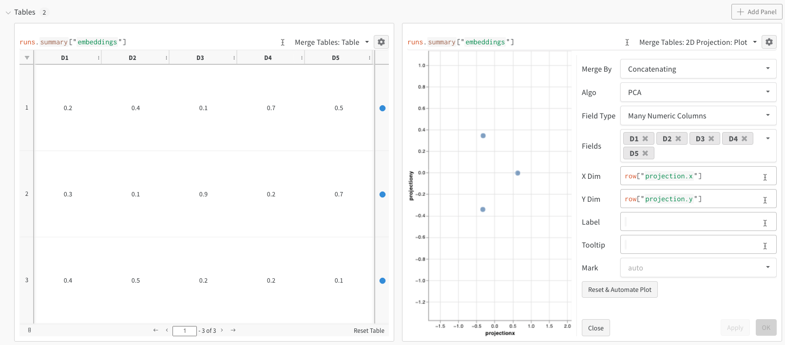
After running the above code, the W&B dashboard will have a new Table containing your data. You can select 2D Projection from the upper right panel selector to plot the embeddings in 2 dimensions. Smart default will be automatically selected, which can be easily overridden in the configuration menu accessed by clicking the gear icon. In this example, we automatically use all 5 available numeric dimensions.

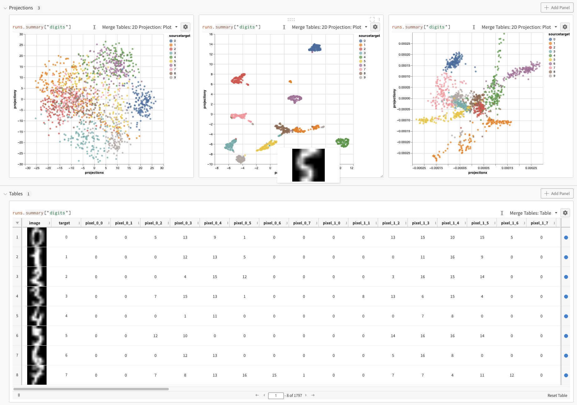
Digits MNIST

While the above example shows the basic mechanics of logging embeddings, typically you are working with many more dimensions and samples. Let’s consider the MNIST Digits dataset (UCI ML hand-written digits datasets) made available via SciKit-Learn. This dataset has 1797 records, each with 64 dimensions. The problem is a 10 class classification use case. We can convert the input data to an image for visualization as well.

import wandb
from sklearn.datasets import load_digits

wandb.init(project="embedding_tutorial")

# Load the dataset
ds = load_digits(as_frame=True)
df = ds.data

# Create a "target" column
df["target"] = ds.target.astype(str)
cols = df.columns.tolist()
df = df[cols[-1:] + cols[:-1]]

# Create an "image" column
df["image"] = df.apply(
    lambda row: wandb.Image(row[1:].values.reshape(8, 8) / 16.0), axis=1
)
cols = df.columns.tolist()
df = df[cols[-1:] + cols[:-1]]

wandb.log({"digits": df})
wandb.finish()

After running the above code, again we are presented with a Table in the UI. By selecting 2D Projection we can configure the definition of the embedding, coloring, algorithm (PCA, UMAP, t-SNE), algorithm parameters, and even overlay (in this case we show the image when hovering over a point). In this particular case, these are all “smart defaults” and you should see something very similar with a single click on 2D Projection. (Click here to interact with this example).

Logging Options

You can log embeddings in a number of different formats:

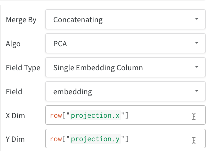
1. Single Embedding Column: Often your data is already in a “matrix”-like format. In this case, you can create a single embedding column - where the data type of the cell values can be list[int], list[float], or np.ndarray.
2. Multiple Numeric Columns: In the above two examples, we use this approach and create a column for each dimension. We currently accept python int or float for the cells.

Furthermore, just like all tables, you have many options regarding how to construct the table:

1. Directly from a dataframe using wandb.Table(dataframe=df)
2. Directly from a list of data using wandb.Table(data=[...], columns=[...])
3. Build the table incrementally row-by-row (great if you have a loop in your code). Add rows to your table using table.add_data(...)
4. Add an embedding column to your table (great if you have a list of predictions in the form of embeddings): table.add_col("col_name", ...)
5. Add a computed column (great if you have a function or model you want to map over your table): table.add_computed_columns(lambda row, ndx: {"embedding": model.predict(row)})

Plotting Options

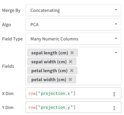
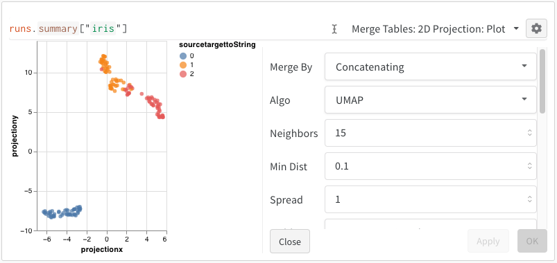
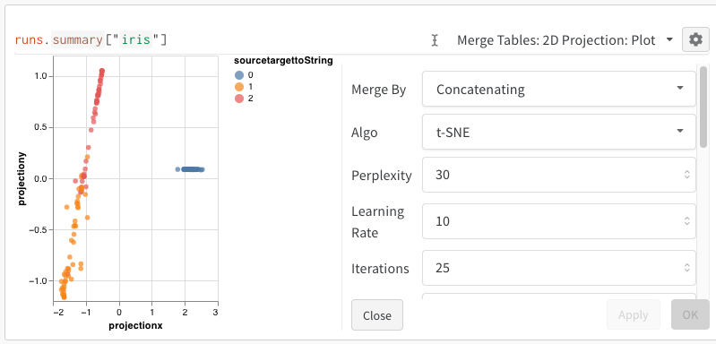
After selecting 2D Projection, you can click the gear icon to edit the rendering settings. In addition to selecting the intended columns (see above), you can select an algorithm of interest (along with the desired parameters). Below you can see the parameters for UMAP and t-SNE respectively.